How Does an Axion Detector Work?

Last month the experiment I worked on as a graduate student published its latest results in Nature. The paper describes how we¹I’m one of 24 authors on this paper, but the true heroes of the story are grad students Kelly Backes and Daniel Palken. My authorship reflects my work getting the initial version of the detector up and running, helping to refine the theoretical formulation of the squeezing concept, and helping to write the manuscript. used the HAYSTAC detector to conduct the first quantum-enhanced search for dark matter in the form of axions.

I’ll forgive you if your first reaction to this brief description is skepticism. Quantum is quite the buzzword these days, and stories about dark matter are seriously overrepresented in popular physics writing. But there is an important result here — it’s not the non-discovery of dark matter, but rather the demonstration of a new application for emerging quantum technologies that are rapidly becoming more and more powerful. I wrote a non-technical article for The Conversation explaining what this result means and why it matters.

This blog post is meant to serve as a companion piece to that article that explains how axion dark matter detectors like HAYSTAC work in more detail. We’ll look under the hood to see what all the parts of the detector are doing, and how its sensitivity is limited by the laws of quantum mechanics. What my colleagues on the HAYSTAC team did to evade this quantum limit in our new result is a rather more complex topic that will have to wait for another time. At the end of the post I’ll discuss the future prospects for the axion dark matter search. You shouldn’t despair, but please don’t hold your breath!

What is dark matter?

We won’t need to know a lot about dark matter for this post, which is fortunate, because physicists don’t know all that much about dark matter either.²Apologies to astronomers, who know a good deal more about dark matter than particle physicists. On a galactic scale, dark matter behaves pretty much like regular matter (stars, interstellar gas clouds, planets, and the like). It exerts a gravitational pull on everything around it and feels the gravitational pull of everything in return.

Observationally, what distinguishes dark matter from regular matter is that it doesn’t appear to have non-gravitational interactions: for instance, it doesn’t emit or absorb light. Dark matter is also extremely abundant. It makes up 85% of the matter in the universe, and it’s spread through galaxies rather uniformly, like a dilute fog. It passes through us constantly without leaving a trace as our solar system orbits the center of the galaxy.

The most intriguing thing about dark matter is that it isn’t made of atoms or other known particles, which means there must be at least one new fundamental particle we haven’t discovered yet. Theoretical particle physicists have cooked up dozens of hypothetical particles, any of which could explain dark matter. Each of these dark matter theories predicts specific extremely weak interactions between dark matter and regular matter — far too feeble to influence astrophysical dynamics, but potentially observable in sufficiently sensitive terrestrial detectors.

Basically, experimental physicists in this field build detectors hyper-sensitive to specific interactions and wait to see if they pick up a signal. If they do — and if they can prove that the signal is not due to something else — somebody gets a Nobel prize. If there’s no signal, we add one more item to the growing list of nonexistent things that aren’t dark matter. To date, no claim of detection has survived scrutiny.

For further reading on how we know what we know about dark matter, independent of what it’s made of, this is a good non-technical introduction.

Dark matter as a cosmic wave

The axion is one of the hypothetical particles that might constitute dark matter. Axions are particularly attractive dark matter candidates because we have another totally unrelated reason to suppose they might exist: the existence of the axion would also resolve a mystery in particle physics called the strong CP problem. I won’t talk about the particle physics motivation for axions further here, but if you’re interested you can check out the first chapter of my thesis, which was written for an audience of non-physicists.

If dark matter is made of axions, it behaves more like an invisible cosmic wave oscillating at a specific frequency than like a bunch of individual particles. As we’ll see below, to detect this wave we will need to know its oscillation frequency, which is proportional to the mass of the axion particle.³This relationship is an example of the quantum phenomenon known as wave-particle duality. But if we set aside the question of why the axion wave has the frequency it does, nothing about its behavior is in any meaningful sense quantum. To use an imperfect analogy, axion dark matter is like the ocean: it manifests as a wave, although at a microscopic level it is really made of a bunch of particles. Unfortunately, the range of possible masses that the axion particle could have (if it even exists) is utterly enormous. As a result, the axion wave frequency could lie anywhere between 300 hertz⁴One hertz is one complete oscillation cycle per second. I wrote about units of measurement (and far too many other things) here. and 300 gigahertz (300 billion hertz).⁵People will sometimes claim that the axion frequency must lie in a smaller fraction of this range, but theoretical arguments to back up this claim admit loopholes. Here I’ve cited the widest range of frequencies the axion could have if it solves the strong CP problem. If we abandon this latter condition and consider the possibility that dark matter might be made of more general axion-like particles, the frequency range is wider still.

To get a more visceral sense of how enormous this range is, imagine you wanted to know the length of some object and I told you it was larger than half an inch but smaller than the diameter of the earth. To date, the vast majority of the axion frequency range remains totally unexplored.

The axion haloscope: a cosmic radio receiver

HAYSTAC is an example of a type of axion detector called a haloscope. Haloscopes search for axion dark matter in a rather small fractional slice⁶As we’ll see later on, when comparing different parts of the axion frequency range, it’s most appropriate to think in fractional rather than absolute terms. In a fractional sense, the 1 – 2 gigahertz frequency range is just large as the 4 – 8 gigahertz range, even though in an absolute sense the latter is four times larger. In each case, the two ends of the range are separated by a factor of two. of the total axion frequency range, 300 megahertz (300 million hertz) to 15 gigahertz or so.⁷Any given haloscope will only be sensitive to signals in an even smaller fraction of this range. HAYSTAC is designed to operate between 4 and 8 gigahertz. Other kinds of detectors are more appropriate for other parts of the range; this was one detail I glossed over in the interest of simplicity in my article for The Conversation.

In that article I explained the basic operation of a haloscope detector using an analogy to a radio receiver. Haloscopes aim to convert axion waves to electromagnetic waves, just as radio receivers convert radio waves to sound waves. They must be tuned over a range of frequencies to find the signal of interest. And the signal (if it exists) is so weak that it will be hard to pick out in the presence of electromagnetic fluctuations akin to radio static.

The electromagnetic wave generated in a haloscope by axion dark matter would oscillate at the same frequency as the axion wave. Electromagnetic waves with frequencies in the 300 megahertz – 15 gigahertz range are called microwaves; they are useful for many other things besides reheating your dinner, with wireless networks being one prominent example.

At this point, I’ll stop talking about waves and instead start describing how haloscopes work using the somewhat more abstract language of fields. This is a pretty good short introduction to fields by a man with a very soothing accent, and if you’re hungry for more about fields at a slightly higher level, you can’t do better than this blog post on the subject by Matt Strassler. Electromagnetic waves are basically electric field oscillations that propagate through space, like ripples spreading out over the surface of a pond; similarly, we can think of axion waves as oscillations of an axion field filling the galaxy. In this post we will be concerned with field oscillations that don’t propagate, but instead stay confined to the same region of space.

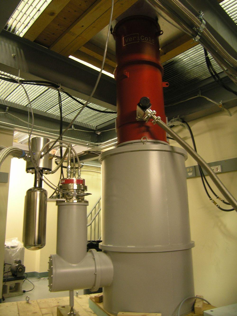
With these preliminaries out of the way, we’re ready to explore how a haloscope works! A haloscope is a tunable microwave cavity immersed in a large magnetic field, maintained at an ultracold temperature, and measured using an exquisitely sensitive amplifier. In the following sections I’ll explain the meaning and relevance of each of the bolded terms here.

[Redacted] magnets: how do they help?

Since the end of the nineteenth century, physicists have known that electric and magnetic fields are intimately connected: for example, a changing magnetic field generates an electric field. If axions exist, the axion field also influences the behavior of electric and magnetic fields. Specifically, an oscillating axion field will generate a tiny electric field oscillating at the same frequency in any region of space where the axion field overlaps with a constant magnetic field.

If dark matter is made of axions, there’s an oscillating axion field permeating all space in the galaxy, which means even your refrigerator magnets are in principle generating a measurable signature of axion dark matter. But there’s a big difference between measurable in principle and measurable in practice: the axion-induced electric field in the vicinity of a fridge magnet would be about a billion billion times weaker than the electric field between the terminals of a nine-volt battery. You’re not going to nab that dark matter Nobel prize for an experiment you conduct in your kitchen.

One way to produce a large magnetic field is to use a type of magnet called a solenoid. A solenoid is a wire wound into a tight coil with a large electric current flowing through it; this current produces a magnetic field in the cylindrical volume inside the coil, which is called the bore of the magnet. If you’ve ever had an MRI, you’ve been inside the bore of a very large solenoid. The magnets used in haloscopes (and MRI scanners) are solenoids with superconducting wires. Superconductors are materials in which electricity can flow without any resistance; this enables the wires to support extremely large currents.

The HAYSTAC magnet generates a 9 tesla magnetic field, about 2000 times stronger than the field of a fridge magnet and six times stronger than that of an MRI scanner, in a bore volume that is roughly 5” in diameter and 10” tall. But even in this strong magnetic field the axion-induced electric field is still far too weak to measure in any reasonable time. To have any hope of detecting it, we need to arrange for this electric field to build up coherently over time using a type of resonator called a microwave cavity.

Resonating with dark matter

Resonance is among the most ubiquitous and practically useful phenomena in physics, and the subject is far too rich to do justice in one section of one blog post. If you’re interested (and you should be!), I wrote an explainer on the subject for Quanta magazine, as well as a blog post on one aspect of the phenomenon. For the purposes of this post, a resonator is a physical system that is very sensitive to external influences that oscillate at a particular frequency, and insensitive to stimuli oscillating at other frequencies.

A simple example of a resonator is a pendulum of the sort you might see in a grandfather clock. Imagine you come across such a pendulum hanging at rest while in the mood to explore the physics of resonators. You can start the pendulum oscillating at its resonant frequency by giving it a push each time it swings back towards you, even if you don’t push very hard. If you give the pendulum periodic pushes at intervals much longer or much shorter than its period of oscillation, you’ll have much less success. In this example we’ve taken the force on the pendulum to be a series of discrete pushes, but the situation is similar for a continuously oscillating force. If the force oscillates at the pendulum’s resonant frequency, it will push the pendulum around; if not, it won’t.

Outside of physics, the word resonance usually refers to the acoustic phenomenon where certain pitches reverberate especially strongly in an enclosed space. Such acoustic resonances occur for sound waves whose wavelengths match the internal dimensions of the enclosure, which may for example be a room or a musical instrument. The speed of sound relates these resonant wavelengths to the corresponding resonant frequencies.

A microwave cavity is an electromagnetic analog to this kind of acoustic resonator. The cavities used in haloscope detectors are hollow copper cylinders whose inner surfaces are machined and polished very precisely to minimize surface roughness. If something starts the electric field inside the cavity oscillating, these oscillations will persist for a long time only if their frequency coincides with one of the resonances determined by the internal dimensions of the cavity. Larger cavities resonate at lower frequencies, just like a cello resonates at lower frequencies than a violin. Microwave cavities, like acoustic resonators, are objects with many resonant frequencies, but the behavior of any of these resonances is similar to the simpler example of the pendulum. For the rest of this post, I’ll focus on a single resonance of the microwave cavity.⁸For reasons I won’t get into here, only a few of the resonances of any given cavity are useful for axion searches.

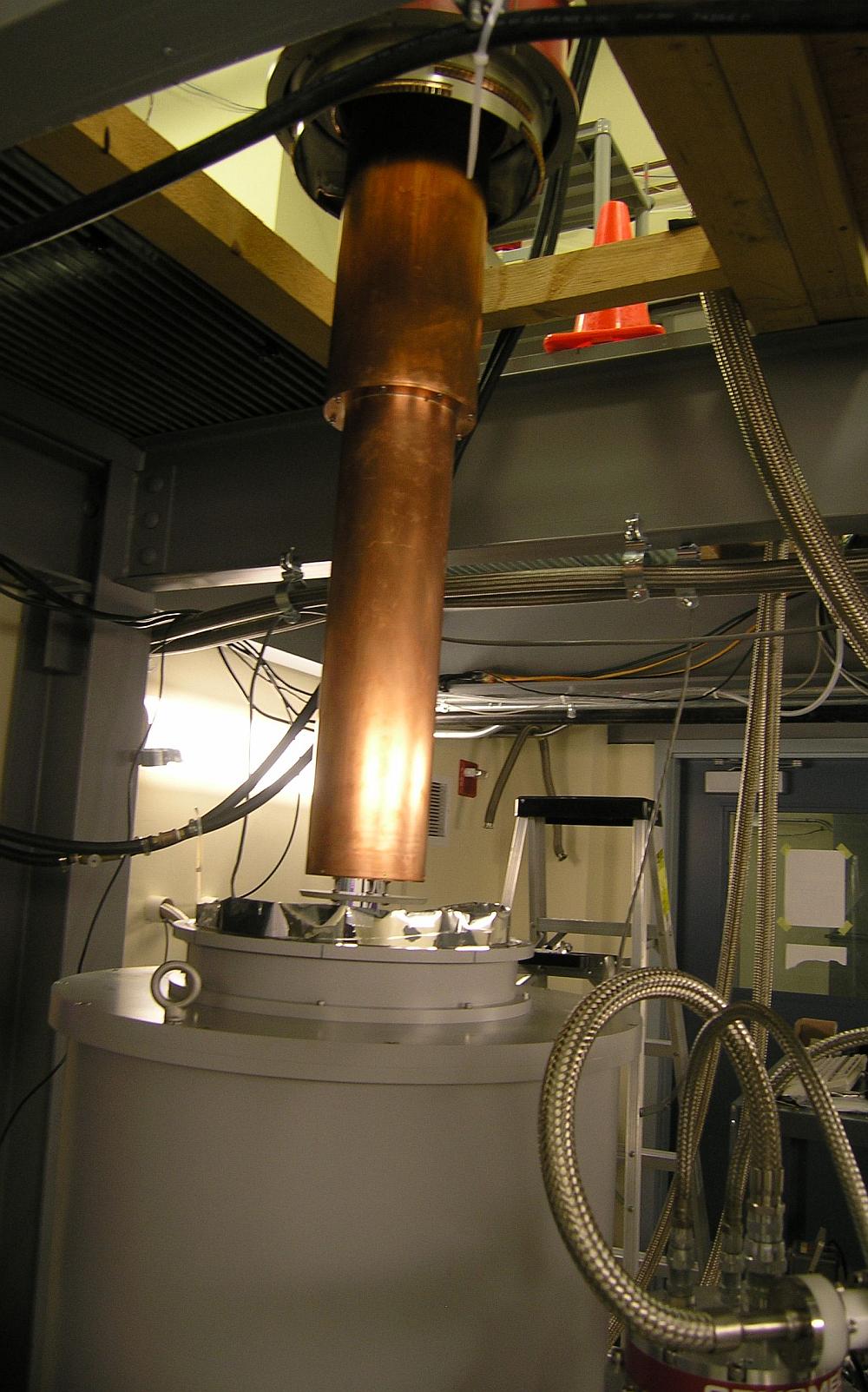
To assemble our haloscope, we hoist the assembly supporting the microwave cavity into the air and slowly lower the cavity into the conveniently cylindrical bore of our magnet. The oscillating electric field produced by axion dark matter would then be enhanced if the axion frequency coincides with the cavity’s resonant frequency. To understand the essential physics, you can think of the cavity as a pendulum, and the axion field as a gentle breeze blowing back and forth at a very regular frequency — the spherical cow of breezes, if you will. The magnetic field in this analogy plays a role similar to the mass of the pendulum. Increasing the magnetic field is like reducing the pendulum mass, making it easier for the wind to push the pendulum around. But whatever its mass, the pendulum will respond most strongly to a force oscillating at its resonant frequency.

If the wind happens to be blowing at this frequency, the amplitude of the pendulum’s oscillations will steadily increase as time goes on. You might wonder where this process stops — surely the motion of the pendulum cannot keep growing forever if the wind keeps blowing. The answer is that there will inevitably be some way for the pendulum to lose energy: friction in the hinge, for instance. This energy loss will balance the incoming energy, resulting in oscillations with some fixed amplitude.

From this analogy, we can see that we want our microwave cavity to lose energy very slowly, so the axion-induced electric field inside will build up for a long time. The rate at which energy leaves a resonator can be expressed in terms of a number called the quality factor, denoted by the symbol \(Q\). A high-\(Q\) resonator continues oscillating for a long time (roughly \(Q\) oscillation cycles) after external forces cease to act on it: a familiar example is a bell that continues ringing audibly for some time after being struck. The microwave cavities used in HAYSTAC has \(Q \sim\) 20,000, limited by the electrical resistance of the copper walls.

We’re now in a position to quantify just how small the axion signal in a haloscope would be, assuming the resonant frequency of the microwave cavity happens to match the axion frequency. In addition to the magnetic field strength and the cavity’s quality factor, the size of the signal also depends on the cavity volume: there’s just more dark matter passing through a larger cavity at any given time. With the state-of-the-art magnet and cavity technology used in HAYSTAC, the signal power — basically, the flow of energy from the axion field into the detector — could be as small as half a yoctowatt, where a yoctowatt is a trillionth of a trillionth of a watt. That’s 0.0000000000000000000000005 watts!

Put another way, if we discover axion dark matter, a hundred trillion trillion haloscopes, covering an area about twice as large as the area enclosed by the orbit of Pluto, would generate enough power for a single light bulb! Feel free to triumphantly present this example to anybody who tells you that particle physics research has no practical applications.

Tuning the dark matter radio

Let’s pause here to review what we’ve learned. Haloscope detectors aim to convert axion field oscillations into electric field oscillations with the same frequency. They use high-\(Q\) microwave cavities in intense magnetic fields to boost these electric field oscillations from hopelessly small to merely agonizingly small.

But the enhancement of the signal by the microwave cavity only works if the cavity’s resonant frequency happens to coincide with the axion frequency — without this enhancement, we’re back to hopelessly small. So to discover or rule out the existence of axion dark matter we must tune the resonant frequency of the cavity. Recall that the distances between metal surfaces inside the cavity determine its resonant frequencies. We can tune the resonance of interest by rotating a copper rod inside the cavity to vary one of these internal dimensions.

So far, I have presented resonance as a phenomenon that occurs at a single frequency. But in practice every resonator has a bandwidth: a narrow frequency window centered on the resonant frequency, within which it will respond strongly. So how narrow are we talking? If a pendulum has a resonant frequency of 1 hertz, will it respond strongly to a force oscillating at 1.1 hertz? What about 1.001 hertz? 1.000001 hertz?

The bandwidth of a resonator turns to be intimately related to its quality factor; more precisely, the bandwidth is equal to the resonant frequency divided by \(Q\).⁹This relationship is the focus of my blog post about resonance, which describes this physics in terms of a resonator’s lifetime \(\tau\) rather than its quality factor \(Q\). \(\tau\) quantifies how long (in seconds) a resonator rings after it’s struck, while \(Q\) is just the lifetime expressed as a number of oscillation cycles. We’ll want to tune our cavity in steps somewhat smaller than its bandwidth, so that adjacent steps will be sensitive to overlapping slices of the possible axion frequency range, and we can be sure that we are not leaving any gaps in our coverage.

This means conducting an axion search with a high-\(Q\) cavity will require a lot of steps: at least \(2Q \sim\) 40,000 to scan through a factor of two in frequency.¹⁰Now we’re in a position to see why it’s best to think in terms of fractional rather than absolute frequency ranges when comparing different detectors. A resonator with a given quality factor will take roughly \(2Q\) steps to scan through a factor of two in frequency, whether this factor of two spans 1 – 2 gigahertz or 4 – 8 gigahertz. Imagine if your car radio had access to this many stations! Unfortunately, nature forgot to supply the programming. At most one and very possibly none of these stations have any content worth listening to.

Sound and fury, signifying nothing

With so many tuning steps required to cover even this tiny fraction of the axion frequency range, we can’t afford to spend much time at each step.¹¹It may seem perverse to use such a high-\(Q\) resonator when there’s such a vast frequency range to cover, but the resonant enhancement of the signal will enable us to spend less time at each tuning step, which more than compensates for the reduced frequency step size. So what determines the required time at each tuning step? Either there is an axion signal or there isn’t. Why can’t we just move on as soon as we measure nothing?

Alas, one never really measures nothing in experimental physics. The question we must always ask is how large we expect the signal to be compared to the noise that is present even in the absence of a signal. In physics and engineering, noise is a generic term for random fluctuations in a measured quantity that can obscure a signal of interest. The radio analogy is again helpful here: the noise is the static that makes it hard to pick out a faint broadcast you hear when you are nearly out of the range of a particular radio station.

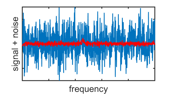
In a haloscope detector, noise will affect the measurement of the electric field in the microwave cavity. We can quantify how much we expect this field to fluctuate at any given frequency without an axion signal. If there is an axion signal, these fluctuations will be larger at the axion frequency than at nearby frequencies. But the noise is random: it is larger at some frequencies than others even in the absence of a signal. By continuously measuring the fluctuating electric field and averaging for a long time, we can make the signal peek out above the noise background: this averaging is what haloscopes do between tuning steps. The more noise there is, the more averaging will be required.

Sources of noise

So much for the effects of noise in a haloscope — where does this noise come from? One important source of noise is related to the temperature of the microwave cavity. On a microscopic level, the temperature of a gas or liquid is a measure of the random motions of its constituent molecules. Similarly, the electrons in the copper walls of the cavity don’t just sit still; rather, they are constantly jittering about, producing fluctuating electric currents that in turn generate fluctuating electric fields inside the cavity. We refer to these fluctuations as thermal noise.

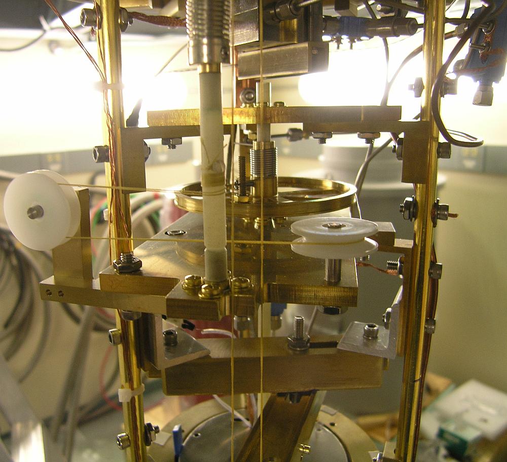
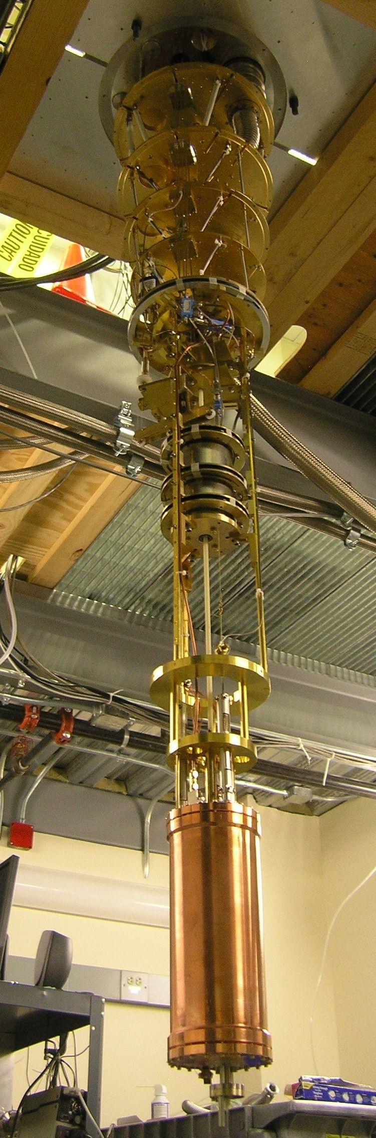
We can minimize thermal noise by cooling the cavity to extremely low temperatures. We use an apparatus called a dilution refrigerator to reach a temperature of about 0.1 degrees Celsius above absolute zero. The HAYSTAC dilution refrigerator is the stack of five gold plates you can see at the top of the picture below; the cavity hangs from the lowest and coldest plate. The physics of dilution refrigerators (and cryogenic experiments more generally) is itself a fascinating subject that will have to wait for another post. To understand how a haloscope works, we don’t need to know about the inner workings of the dilution refrigerator; its role is just to make the cavity and other critical parts of the detector very cold.

Unfortunately, getting rid of thermal noise is not the whole story. It’s all very well to make the cavity extremely cold, but at some point we have to measure the electric field in the cavity, and the act of measurement itself can introduce noise in several distinct ways. Noise introduced by measurement is a remarkably subtle subject — one I daresay is not always appreciated by scientists working in this field. Let’s add it to the growing list of topics for future posts. Here I’ll focus on one specific form of measurement-related noise: the noise added by the extremely sensitive cryogenic amplifiers used in haloscope detectors.¹²For the purposes of this post, an amplifier is an electronic circuit that increases the size of a signal without changing any of its frequencies. The volume knob in a car stereo is a good example. As you turn up the volume, the audio gets louder but isn’t distorted.

The amplification of weak signals is a routine task in experimental physics, and amplifier added noise may seem like something we should be able to avoid with sensible experimental design. If amplifiers add noise, why do we need to use an amplifier at all? Let’s imagine there really is an axion field oscillating at the resonant frequency of our cavity. To detect the axion signal, we need to extract it from the cavity, bring it back up to room temperature, and feed it into a computer to record and process the data. Transporting the signal is a lossy process — only a small fraction of the signal power will make it all the way up to room temperature, with the rest being lost to the electrical resistance of cables and electronic components used to route the signal.¹³Cables with higher electrical conductivity also generally have higher thermal conductivity, and can prevent the dilution refrigerator from getting down to its minimum temperature. To make matters worse, this heavily attenuated signal has to compete with much larger noise at higher temperatures.

We can avoid these problems by putting a very sensitive amplifier as close to the cavity as possib­­le: once the signal has been amplified by a factor of 1000 or so, it doesn’t really matter if it’s subsequently attenuated by a factor of 10. But it’s not possible to amplify the signal an axion would generate in the cavity without also amplifying the cavity thermal noise. This means amplification can never increase the ratio of signal to noise, which is what really determines haloscope sensitivity, and amplifier added noise will always reduce this ratio! You can think of amplification like car insurance: you pay a little bit in signal-to-noise ratio upfront to avoid paying through the nose later in the measurement process.¹⁴I first heard this analogy from Rob Schoelkopf.

To the quantum noise limit

We’ve again reached a good point to pause and summarize what we’ve learned in the last few sections. Noise in the form of random electric field fluctuations determines how long a haloscope must average at each tuning step to resolve any axion signal that might be present. We’ve discussed two important contributions to this noise: thermal noise associated with the temperature of the microwave cavity and noise added by the amplifier required to measure such a weak signal.

So how small can we make this noise? This is where quantum mechanics finally enters the story, and it comes bearing bad news. Make the cavity as cold as you like and use the world’s best amplifiers — you won’t be able to reduce the noise in a haloscope below a fundamental minimum level called the standard quantum limit.

The standard quantum limit is a consequence of the law of quantum mechanics known as Heisenberg’s uncertainty principle. The uncertainty principle states that it is impossible to know the exact values of certain pairs of physical quantities at the same time. The position and momentum of a particle are the most commonly cited examples of quantities that cannot be known simultaneously.

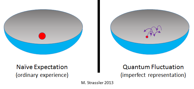
Let’s consider the example of a marble rolling around near the bottom of a bowl. If the marble behaved like a quantum particle, you could never be sure that it was sitting still at the bottom of the bowl. Moreover, if you tried to continuously monitor the marble’s position it would appear to move around randomly within some small region near the bottom. This random apparent motion isn’t just a consequence of imperfect measurement: if your measurement indicated that the marble’s position wasn’t fluctuating, you’d know exactly where the marble was and also know that it wasn’t moving, in violation of the uncertainty principle. We can think of this random apparent motion as noise affecting the measurement of the marble’s position. In the same way, the uncertainty principle gives rise to noise in a continuous measurement of the electric field in a haloscope detector.¹⁵To more formally describe how the uncertainty principle gives rise to the standard quantum limit, we’d need to introduce two rather abstract quantities called field quadratures, which represent two complementary ways that the electric field can oscillate at any frequency. These quadratures play the role of the marble’s position and momentum in the analogy above; they are the two quantities that can’t be simultaneously measured.

The main result of my PhD research was reducing the noise in HAYSTAC to near the standard quantum limit, by integrating a superconducting circuit called a Josephson parametric amplifier (JPA) into the detector. JPAs are widely used in quantum computing research; they are ideal amplifiers, which is to say that if their added noise were any smaller it would violate the uncertainty principle.¹⁶The minimum noise at the standard quantum limit can be attributed in part to the apparent fluctuations in the electric field discussed above and in part to additional noise introduced by a measurement of this field with an ideal amplifier; both contributions are consequences of the uncertainty principle. But this is getting further into the weeds than necessary for the present discussion. This post is already very long, so I’ll spare you the details of how JPAs work and what technical hurdles we had to overcome to incorporate one into HAYSTAC. Perhaps another time!

I said above that an axion signal in HAYSTAC could be as small as half a trillionth of a trillionth of a watt. But we don’t actually want to fill the solar system with haloscopes to power a light bulb. Instead we should ask how large the signal would be compared to noise at the standard quantum limit. The noise turns out to be 30,000 times larger, and more than two months of averaging at each step would be required to resolve the signal or definitively rule it out. Scanning a factor of two in frequency at this rate would take more than seven thousand years!

Is it hopeless?

Numbers like this should make us stop and reflect on whether we know what we’re doing. Should I regret devoting five years of my life to the search for axion dark matter? How many grad students are we willing to sacrifice to the dark and possibly nonexistent god of the axion?

Even in the face of these grim numbers, there is reason for tempered optimism. Frequency scan rates have increased by nearly a factor of a million since the first haloscope started operating in 1987.¹⁷This doesn’t mean that early haloscopes actually averaged for a million months at each tuning step, or for that matter that present-day haloscopes sit at the same step for a month. Rather, most haloscopes have scanned faster to rule out theories in which the axion’s electromagnetic interaction is stronger than the minimum value I’ve assumed throughout this post. The first prototype haloscope would have needed to scan a million times slower than HAYSTAC to achieve the same sensitivity as we do today. Further speedups will be hard-fought now that the low-hanging fruit has been picked. But our latest result in Nature has demonstrated the promise of quantum noise manipulation techniques for improving haloscope scan rates, and the requisite quantum technology is maturing rapidly. Complementary detector upgrades aim to increase the signal power rather than reduce the noise, using synchronized arrays of many cavities and more powerful magnets.¹⁸Recall that lower-frequency resonators have larger volumes (think cello vs. violin) and that the signal power is proportional to the cavity volume — there’s just more dark matter in a bigger cavity. For this reason, haloscopes searching at lower frequencies than HAYSTAC can scan a lot faster, and the situation is even worse for haloscopes searching at higher frequencies. Cavity arrays offer one promising path to increasing detector volumes, but making them work with dozens or hundreds of cavities is a very difficult engineering problem. None of these upgrades alone will enable a comprehensive scan of the full axion frequency range any time soon. But with simultaneous advances on several fronts it’s reasonable to hope that the total scan time will be measured in decades rather than millennia.

In my view it’s better to think of today’s haloscopes as prototypes for the development of technologies essential to future detectors than as dark matter detectors themselves — of course they could discover dark matter, but by the same token you could win the lottery tomorrow. Unfortunately the ecosystem of research funding and popularization tends to incentivize more dramatic statements about the possibility of detection. We shouldn’t give up on the search for dark matter, but a pattern of bold claims followed by non-detection can undermine public confidence in the scientific endeavor. One of the chief lessons of modern cosmology is that there’s a lot we still don’t understand about the workings of nature. We would do well to approach the dark matter search with a little intellectual humility.